Acoustic S-Matrices for plane waves

In addition to the T-matrix method, where incident and scattered fields are related, S-matrices relate incoming and outgoing fields. To describe scattering in the plane wave basis, we use exactly such a S-matrix description. The incoming and outgoing waves are defined with respect to a plane, typically the xy plane. This plane additionally separates the whole space into two parts. This then separates the description into four parts: the transmission of fields propagating in the positive and negative z direction, and the reflection of those fields.

Slabs

The main object for plane wave computations is the class AcousticSMatrices which exactly collects those four individual S-matrices. For simple interfaces and the propagation in a homogeneous medium these S-matrices can be obtained analytically. Combining these two objects then allows the description of simple slabs.

k0s = 2 * np.pi * np.linspace(1000, 300000, 100) / 343
materials = [(798, 1050), (1050, 2350), (998, 1497)]
thickness = 0.005
tr = np.zeros((2, len(k0s)))

def compute_coeffs(k0):
    pwb = acoustotreams.ScalarPlaneWaveBasisByComp.default([0, 0.1 * k0])
    slab = acoustotreams.AcousticSMatrices.slab(thickness, pwb, k0, materials)
    return slab.tr([1])
tr = np.array(
    Parallel(n_jobs=-1)(delayed(compute_coeffs)(k0s[i]) for i in range(len(k0s)))
)

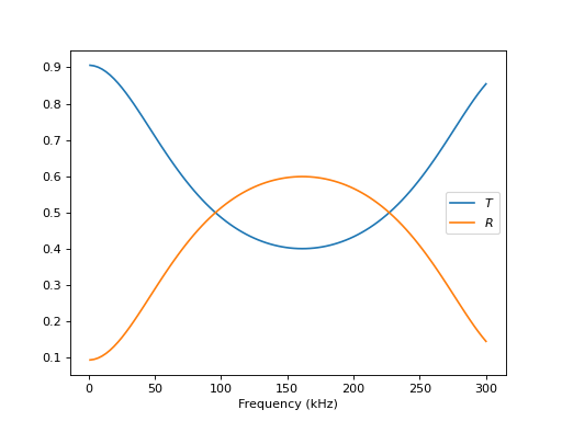
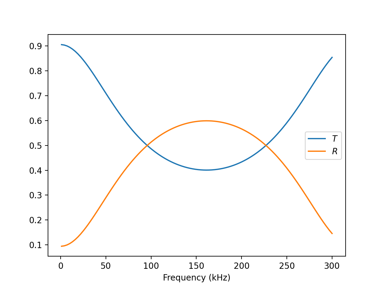
The setup is fairly simple. The materials are given in order from negative to positive z coordinates. We simply loop over the wave number and calculate transmission and reflection.

(Source code, png, hires.png, pdf)

From T-matrix arrays

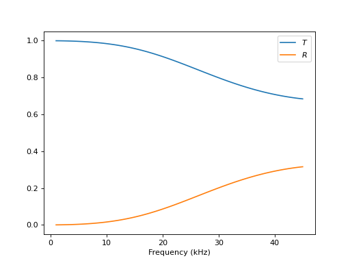
While this example is simple we can build more complicated structures from two-dimensional arrays of T-matrices. We take spheres on an thin film as an example. This means we first calculate the S-matrices for the thin film and the array individually and then couple those two systems.

k0s =  2 * np.pi * np.linspace(1000, 45000, 100) / 343
material_slab = acoustotreams.AcousticMaterial(698, 950)
thickness = 0.0025
period = 0.025
lattice = acoustotreams.Lattice.square(period)
materials = [acoustotreams.AcousticMaterial(1050, 2350), 
            acoustotreams.AcousticMaterial(998, 1497)]
n = 343 / 1497
radius = 0.0075
lmax = 3

Beforehand, we define all the necessary parameters. First the wave numbers, then the parameters of the slab, and finally those for the lattice and the spheres. Then, we can use a simple loop to solve the system for all wave numbers.

tr = np.zeros((len(k0s), 2))
def compute_coeffs(k0):
    kpar = np.array([0, 0.1 * k0])

    spheres = acoustotreams.AcousticTMatrix.sphere(
        lmax, k0, radius, materials
        ).latticeinteraction.solve(lattice, kpar * n)
    
    bmax = 3.1 * 2 * np.pi / period
    spwb = acoustotreams.ScalarPlaneWaveBasisByComp.diffr_orders(kpar * n, lattice, bmax)
    splw = acoustotreams.plane_wave_scalar(kpar * n, k0=k0, basis=spwb, material=materials[1])
    slab = acoustotreams.AcousticSMatrices.slab(thickness, spwb, k0, [materials[1], material_slab, materials[1]])
    dist = acoustotreams.AcousticSMatrices.propagation([0, 0, radius], spwb, k0, materials[1])
    array = acoustotreams.AcousticSMatrices.from_array(spheres, spwb)
    total = acoustotreams.AcousticSMatrices.stack([slab, dist, array])
    return total.tr(splw)
tr = np.array(
    Parallel(n_jobs=-1)(delayed(compute_coeffs)(k0s[i]) for i in range(len(k0s)))
)

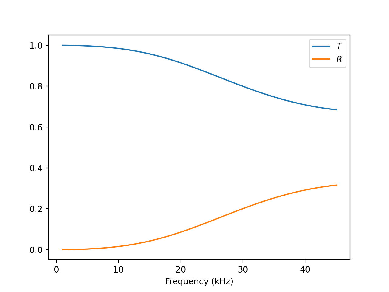
We set an oblique incidence and the array of spheres. Then, we define a plane wave and the needed S-matrices: a slab, the distance between the top interface of the slab to the center of the sphere array, and the array in the S-matrix representation itself.

(Source code, png, hires.png, pdf)

From cylindrical T-matrix gratings

Now, we want to perform a small test of the methods. Instead of creating the two-dimensional sphere array right away, we intermediately create a one-dimensional array, then calculate cylindrical T-matrices, and place them in a second one-dimensional lattice, thereby, obtaining the S-matrix from the previous section.

k0s =  2 * np.pi * np.linspace(1000, 45000, 100) / 343
material_slab = acoustotreams.AcousticMaterial(698, 950)
thickness = 0.0025
period = 0.025
lattice = acoustotreams.Lattice.square(period)
materials = [acoustotreams.AcousticMaterial(1050, 2350), 
            acoustotreams.AcousticMaterial(998, 1497)]
n = 343 / 1497
radius = 0.0075
lmax = mmax = 3

The definition of the parameters is quite similar. We store the lattice period for later use separately and define the maximal order mmax also separately.

tr = np.zeros((len(k0s), 2))
def compute_coeffs(k0):
    kpar = np.array([0, 0.1 * k0])

    spheres = acoustotreams.AcousticTMatrix.sphere(
        lmax, k0, radius, materials
        ).latticeinteraction.solve(period, kpar[0] * n)
    
    bmax = 3.1 * 2 * np.pi / period
    cwb = acoustotreams.ScalarCylindricalWaveBasis.diffr_orders(kpar[0] * n, mmax, period, bmax)
    spheres_tmc = acoustotreams.AcousticTMatrixC.from_array(
        spheres, cwb
    ).latticeinteraction.solve(period, kpar[1] * n)

    spwb = acoustotreams.ScalarPlaneWaveBasisByComp.diffr_orders(kpar * n, lattice, bmax)
    splw = acoustotreams.plane_wave_scalar(kpar * n, k0=k0, basis=spwb, material=materials[1])
    slab = acoustotreams.AcousticSMatrices.slab(thickness, spwb, k0, [materials[1], material_slab, materials[1]])
    dist = acoustotreams.AcousticSMatrices.propagation([0, 0, radius], spwb, k0, materials[1])
    array = acoustotreams.AcousticSMatrices.from_array(spheres_tmc, spwb)

The first half of the loop is now a little bit different. After creating the spheres we solve the interaction along the z direction, then create the cylindrical T-matrix and finally calculate the interaction along the x direction. The second half is the same as in the previous calculation.

The most important aspect to note here, is that the method from_array() implicitly converts the lattice in the zx plane to a lattice in the xy plane.

(Source code, png, hires.png, pdf)

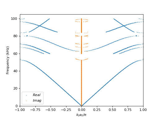
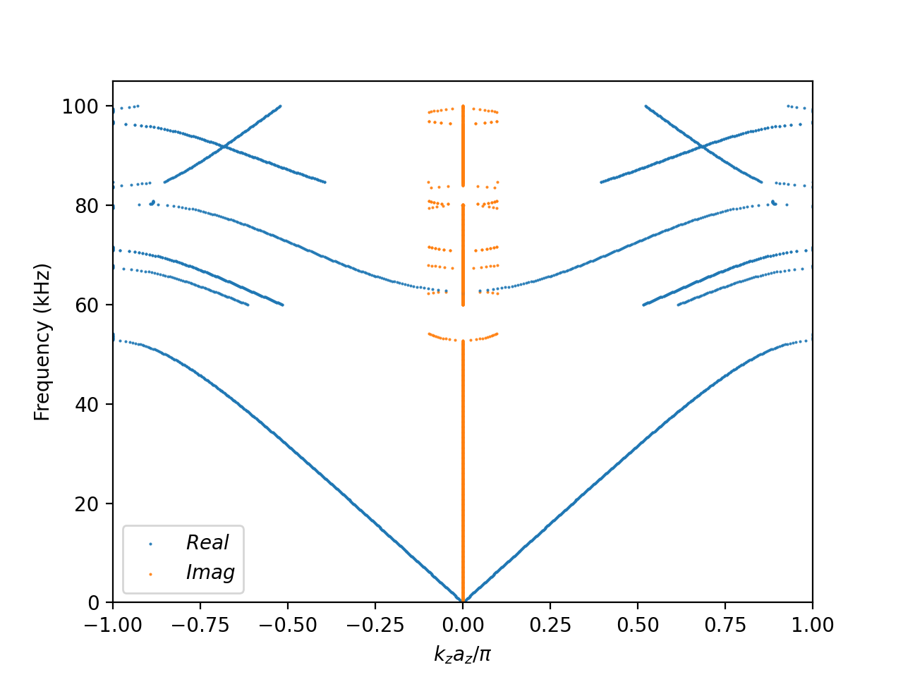
Band structure

Finally, we want to compute the band structure of a system consisting of the periodic repetition of an S-matrix along the z direction. In principle, one can obtain this band structure also from the lattice interaction in the T-matrix, but calculating it from the S-matrix has two benefits. First, more complex systems can be analyzed, because slabs and objects described by cylindrical T-matrices can be included. Second, one only defines \(k_0\), \(k_x\), and \(k_y\). Then, the result of the calculation are all values \(k_z\) and the plane wave decomposition from an eigenvalue decomposition. So, instead of a 4-dimensional parameter sweep only a 3-dimensional sweep is necessary decreasing the computation time. The downside is, that one is restricted to unit cells, where one vector points along the z axis and is perpendicular to the other two.

We take the array of spheres on top of a slab and continue this one infinitely along the z axis. Thus, the setup is

k0s =  2 * np.pi * np.linspace(100, 100000, 800) / 343
material_slab = acoustotreams.AcousticMaterial(698, 950)
thickness = 0.0025
period = 0.025
lattice = acoustotreams.Lattice.square(period)
materials = [acoustotreams.AcousticMaterial(1050, 2350), 
            acoustotreams.AcousticMaterial(998, 1497)]
n = materials[1].c / 343 
radius = 0.0075
lmax = 4
az = 0.02

where az is the length of the lattice vector pointing in the z direction. With a simple loop we can get the band structure for \(k_x = k_y = 0\).

def compute_coeffs(k0):
    kpar = np.array([0, 0])

    spheres = acoustotreams.AcousticTMatrix.sphere(
        lmax, k0, radius, materials
        ).latticeinteraction.solve(lattice, kpar / n)
    
    bmax = 1.1 * 2 * np.pi / period * compute_ndiff(period, 2 * np.pi * n / k0)
    spwb = acoustotreams.ScalarPlaneWaveBasisByComp.diffr_orders(kpar / n, lattice, bmax)
    slab = acoustotreams.AcousticSMatrices.slab(thickness, spwb, k0, [materials[1], material_slab, materials[1]])
    dist = acoustotreams.AcousticSMatrices.propagation([0, 0, radius], spwb, k0, materials[1])
    array = acoustotreams.AcousticSMatrices.from_array(spheres, spwb)
    total = acoustotreams.AcousticSMatrices.stack([slab, dist, array])
    x, _ = total.bands_kz(az)
    x = x * az / np.pi
    return x[np.abs(np.imag(x)) < 0.1]

res = Parallel(n_jobs=-1)(delayed(compute_coeffs)(k0s[i]) for i in range(len(k0s)))

which looks as follows, after a cut on the imaginary part of the \(k_z\) component.

(Source code, png, hires.png, pdf)