Acoustic cylindrical T-Matrices

Here, we cover acoustical cylindrical T-matrices, which are distinguished from the more conventional (spherical) T-matrices through the use of scalar cylindrical waves as the basis instead of scalar spherical waves. These waves are parametrized by the z component of the wave vector \(k_z\), which describes their behavior in the z direction \(\mathrm e^{\mathrm i k_z z}\), and the azimuthal order \(m\), which is also used in scalar spherical waves.

The cylindrical T-matrices are suited for structures that are periodic in one dimension (conventionally set along the z axis). Similarly to T-matrices of spheres that contain the analytically known Mie coefficients, the cylindrical T-matrices for infinitely long cylinders can also be calculated analytically.

Another similarity to spherical T-matrices are the possibilities to describe clusters of objects in a local and global basis and to place these objects in a lattice. The lattices can only extend in one and two dimensions; the z direction is implicitly periodic already.

Infinitely long cylinders

The first simple object, for which we calculate the cylindrical T-matrix is an infinitely long cylinder. Due to the rotation symmetry about the z axis this matrix is diagonal with respect to m and due to the translation symmetry it is also diagonal with respect to kz.

k0s = 2 * np.pi * np.linspace(50000, 500000, 200) / 343
materials = [acoustotreams.AcousticMaterial(1050 + 100j, 2350 - 300j), 
             acoustotreams.AcousticMaterial(998, 1497)]
kzs = [0]
mmax = 10
radius = 0.005
cylinders = [acoustotreams.AcousticTMatrixC.cylinder(kzs, mmax, k0, radius, materials) for k0 in k0s]

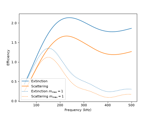
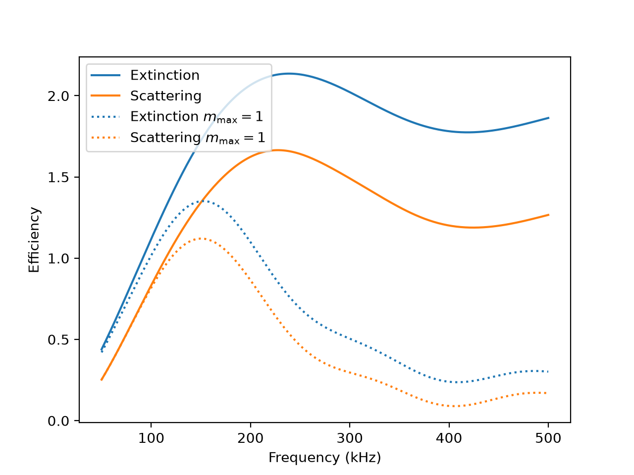
For such infinitely long structures it makes more sense to talk about cross width instead of cross section. We obtain the averaged scattering and extinction cross width by

xw_sca = np.array([tm.xw_sca_avg for tm in cylinders]) / (2 * radius)
xw_ext = np.array([tm.xw_ext_avg for tm in cylinders]) / (2 * radius)

Again, we can also select specific modes only, for example the modes with \(m = 0\) and \(m = \pm 1\).

cwb_mmax0 = acoustotreams.ScalarCylindricalWaveBasis.default(kzs, 1)
cylinders_mmax0 = [tm[cwb_mmax0] for tm in cylinders]
xw_sca_mmax0 = np.array([tm.xw_sca_avg for tm in cylinders_mmax0]) / (2 * radius)
xw_ext_mmax0 = np.array([tm.xw_ext_avg for tm in cylinders_mmax0]) / (2 * radius)

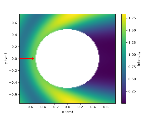
to calculate their cross width. Evaluating the field intensity in the xy plane is similar to the case of a sphere.

tm = cylinders[50]
inc = acoustotreams.plane_wave_scalar([tm.k0, 0, 0], k0=tm.k0, material=tm.material)
sca = tm.sca(inc)

x = np.linspace(-0.0075, 0.0075, 101)
y = np.linspace(-0.0075, 0.0075, 101)
def compute_intensity(i, j):
    r = [x[j], y[i], 0]
    result = 0  
    if tm.valid_points(r, [radius]): 
        result = np.abs(inc.pfield(r) + sca.pfield(r))**2  
    else:
        result = np.nan
    return i, j, result  
results = Parallel(n_jobs=-1)(
    delayed(compute_intensity)(i, j) for i in range(len(y)) for j in range(len(x))
)
intensity = np.zeros((len(y), len(x)))
for i, j, result in results:
    intensity[i, j] = result

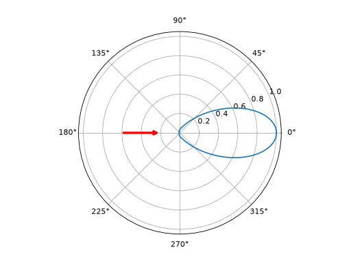
For the infinite cylinder we can also calculate the radiation pattern as a function of the angle \(\varphi\). The red arrow indicates the direction of incidence of the plane wave.

(Source code)

Cylindrical T-matrices for one-dimensional arrays of spherical T-matrices

For our next example we want to look at the system of spheres on a one-dimensional lattice again (One-dimensional arrays (along z)). They fulfil all properties that define structures where the use of cylindrical waves is beneficial, namely they have a finite extent in the xy plane and they are periodic along the z direction.

Thus, the initial setup of our calculation starts with spheres in the spherical wave basis and placing them in a chain. This is the same procedure as in One-dimensional arrays (along z). We define a nonzero component of the wave vector along the z axis \(k_z\) in the air.

k0 =  2 * np.pi * 50000 / 343
materials = [acoustotreams.AcousticMaterial(1050 + 100j, 2350 - 300j), 
            acoustotreams.AcousticMaterial(998, 1497)]
lmax = mmax = 3
radii = [0.0075, 0.0065]
positions = [[-0.004, 0, -0.0075], [0.004, 0, 0.0075]]
period = 0.035
lattice = acoustotreams.Lattice(period)
kz = 0.1 * k0
n = 343 / 1497

spheres = [acoustotreams.AcousticTMatrix.sphere(lmax, k0, r, materials) for r in radii]
chain = acoustotreams.AcousticTMatrix.cluster(spheres, positions).latticeinteraction.solve(lattice, kz * n)

Here we also define \(n\) as a “refractive index” for the background medium of the spheres with respect to the air and divide \(k_z\) by \(n\) when it is needed. Next, we convert this chain in the spherical wave basis to a suitable cylindrical wave basis.

bmax = 3.1 * lattice.reciprocal
cwb = acoustotreams.ScalarCylindricalWaveBasis.diffr_orders(kz * n, mmax, lattice, bmax, 2, positions)
chain_tmc = acoustotreams.AcousticTMatrixC.from_array(chain, cwb)

We chose to add the first three diffraction orders (plus a 0.1 margin to avoid problems with floating point comparisons).

Finally, we set-up the incident wave and calculate the scattering coeffcients by the usual procedure.

inc = acoustotreams.plane_wave_scalar(
    [np.sqrt(chain.k0 * chain.k0 - kz * kz), 0, kz], 
    k0=chain.k0, 
    material=chain.material
)
sca = chain.sca(inc)
sca_tmc = chain_tmc.sca(inc)

We evaluate the fields in two regions. Outside of the circumscribing cylinders we can use the fast cylindrical wave expansion. Inside of the circumscribing cylinders but outside of the spheres we can use the method of One-dimensional arrays (along z).

x = np.linspace(-0.75 * period, 0.75 * period, 101)
z = np.linspace(-0.5 * period, 0.5 * period, 101)
def compute_pressure(i, j):
    r = [x[j], 0, z[i]]  
    if chain_tmc.valid_points(r, radii):
        result = sca_tmc.pfield(r) 
    else:
        result = np.nan
        if chain.valid_points(r, radii):
            swb = acoustotreams.ScalarSphericalWaveBasis.default(0, positions=[r])
            result = sca.expandlattice(basis=swb).pfield(r) 
    return i, j, result  
results = Parallel(n_jobs=-1)(
    delayed(compute_pressure)(i, j) 
    for i in range(len(z)) 
    for j in range(len(x))
)
p = np.zeros((len(z), len(x)), complex)
for i, j, result in results:
    p[i, j] = result

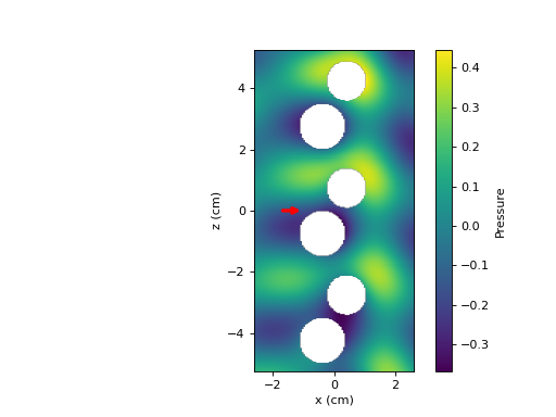
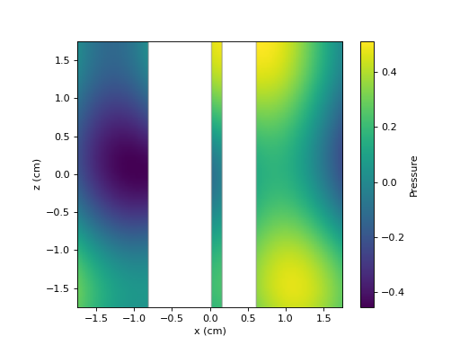
Finally, we can plot the results. To illustrate the periodicity better, three unit cells are shown.

(Source code)

Clusters

Similarly to the case of spheres we can also calculate the response from a cluster of objects. As an example let us simulate a cylinder together with a chain of spheres in the cylindrical wave basis as described in the previous section.

Hence, we set up first the spheres in the chain and convert them to the cylindrical wave basis as before

k0 =  2 * np.pi * 50000 / 343
materials = [acoustotreams.AcousticMaterial(1050 + 100j, 2350 - 300j), 
            acoustotreams.AcousticMaterial(998, 1497)]
lmax = mmax = 3
radii = [0.0065, 0.0055]
positions = [[-0.004, -0.005, 0], [0.004, 0.005, 0]]
period = 0.035
lattice = acoustotreams.Lattice(period)
kz = 0.1 * k0
n = 343 / 1497

sphere = acoustotreams.AcousticTMatrix.sphere(lmax, k0, radii[0], materials)
chain = sphere.latticeinteraction.solve(lattice, kz * n)
bmax = 3.1 * lattice.reciprocal
cwb = acoustotreams.ScalarCylindricalWaveBasis.diffr_orders(kz * n, mmax, lattice, bmax)
chain_tmc = acoustotreams.AcousticTMatrixC.from_array(chain, cwb)

Then, we create the T-matrix of the cylinder in the cylindrical wave basis.

cylinder = acoustotreams.AcousticTMatrixC.cylinder(np.unique(cwb.kz), mmax, k0, radii[1], materials)

Finally, we construct the cluster, find the T-matrix of the interacting system, and then scattered field coeffcients for the incident plane wave.

cluster = acoustotreams.AcousticTMatrixC.cluster([chain_tmc, cylinder], positions).interaction.solve()
inc = acoustotreams.plane_wave_scalar(
    [np.sqrt(cluster.k0 * cluster.k0 - kz * kz), 0, kz], 
    k0=cluster.k0, 
    material=cluster.material
)
sca = cluster.sca(inc)

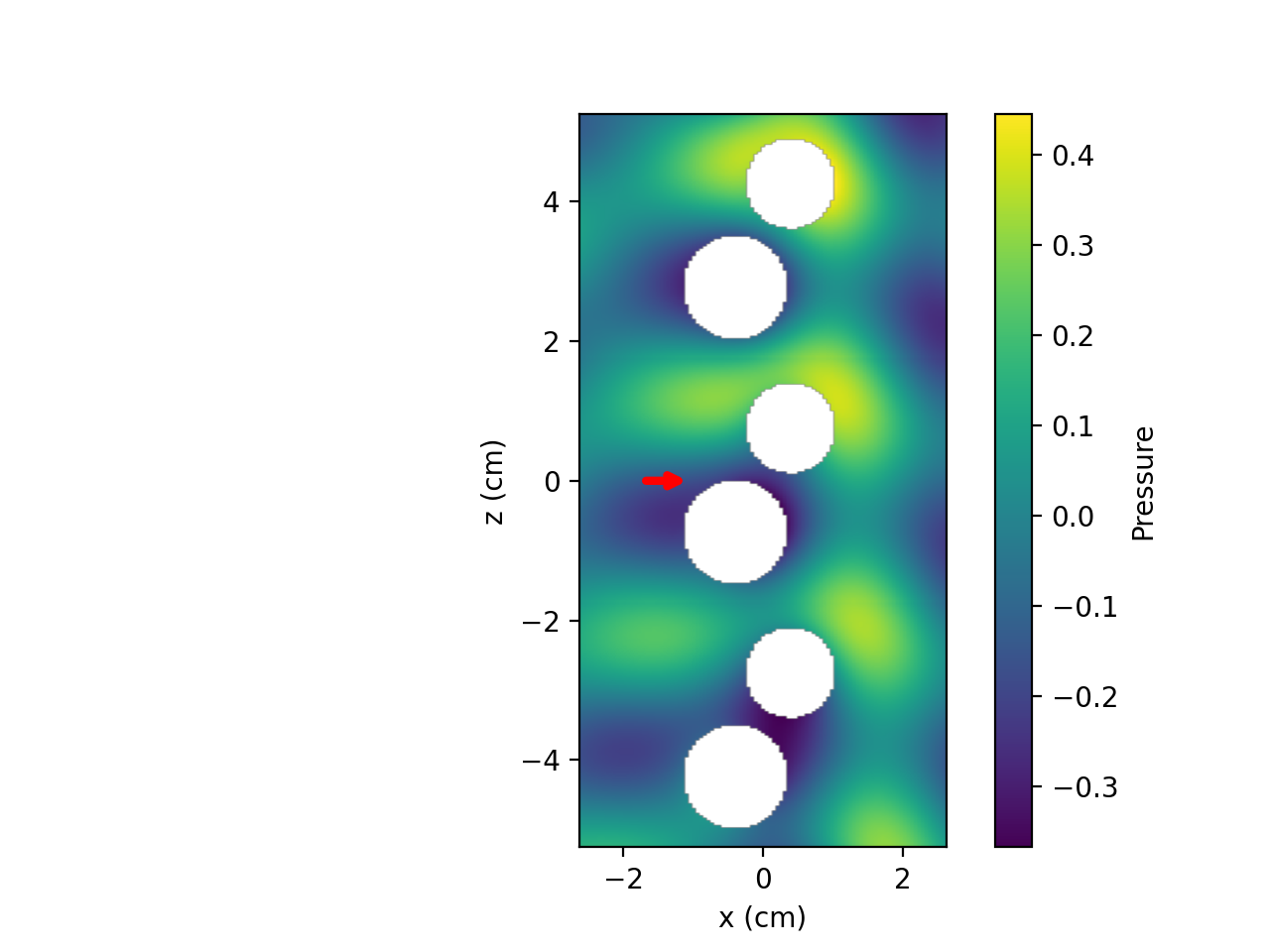
The scattered pressure field within three unit cells is shown below

(Source code)

One-dimensional arrays (along the x axis)

Now, we take the chain of spheres and cylinder and place them in a grating structure along the x direction. We start again by defining the parameters and calculating the relevant cylindrical T-matrices.

k0 =  2 * np.pi * 50000 / 343
materials = [acoustotreams.AcousticMaterial(1050 + 100j, 2350 - 300j), 
            acoustotreams.AcousticMaterial(998, 1497)]
lmax = mmax = 3
radii = [0.0065, 0.0055]
positions = [[-0.004, -0.005, 0], [0.004, 0.005, 0]]
period = 0.035
lattice_z = acoustotreams.Lattice(period)
lattice_x = acoustotreams.Lattice(period, "x")
kz = 0.1 * k0
n = 343 / 1497

sphere = acoustotreams.AcousticTMatrix.sphere(lmax, k0, radii[0], materials)
chain = sphere.latticeinteraction.solve(lattice_z, kz * n)
bmax = 3.1 * lattice_z.reciprocal
cwb = acoustotreams.ScalarCylindricalWaveBasis.diffr_orders(kz * n, mmax, lattice_z, bmax)
kzs = np.unique(cwb.kz)
chain_tmc = acoustotreams.AcousticTMatrixC.from_array(chain, cwb)
cylinder = acoustotreams.AcousticTMatrixC.cylinder(kzs, mmax, k0, radii[1], materials)

Next, we create the cluster and, as usual, let it interact within a lattice of the defined periodicity. Then, we simply calculate the scattering coefficients.

cluster = acoustotreams.AcousticTMatrixC.cluster(
    [chain_tmc, cylinder], positions
).latticeinteraction.solve(lattice_x, 0)
inc = acoustotreams.plane_wave_scalar(
    [0, np.sqrt(cluster.k0 * cluster.k0 - kz * kz), kz], 
    k0=cluster.k0, 
    material=cluster.material
)
sca = cluster.sca(inc)

In the last step, we sum up the scattered fields at each point we want to calculate the pressure field.

x = np.linspace(-0.5 * period, 0.5 * period, 101)
z = np.linspace(-0.5 * period, 0.5 * period, 101)
def compute_pressure(i, j):
    r = [x[j], 0, z[i]]  
    if cluster.valid_points(r, radii):
        cwb = acoustotreams.ScalarCylindricalWaveBasis.default(kzs, 0, positions=[r])
        result = sca.expandlattice(basis=cwb).pfield(r)
    else:
        result = np.nan
    return i, j, result  
results = Parallel(n_jobs=-1)(
    delayed(compute_pressure)(i, j) 
    for i in range(len(z)) 
    for j in range(len(x))
)
p = np.zeros((len(z), len(x)), complex)
for i, j, result in results:
    p[i, j] = result

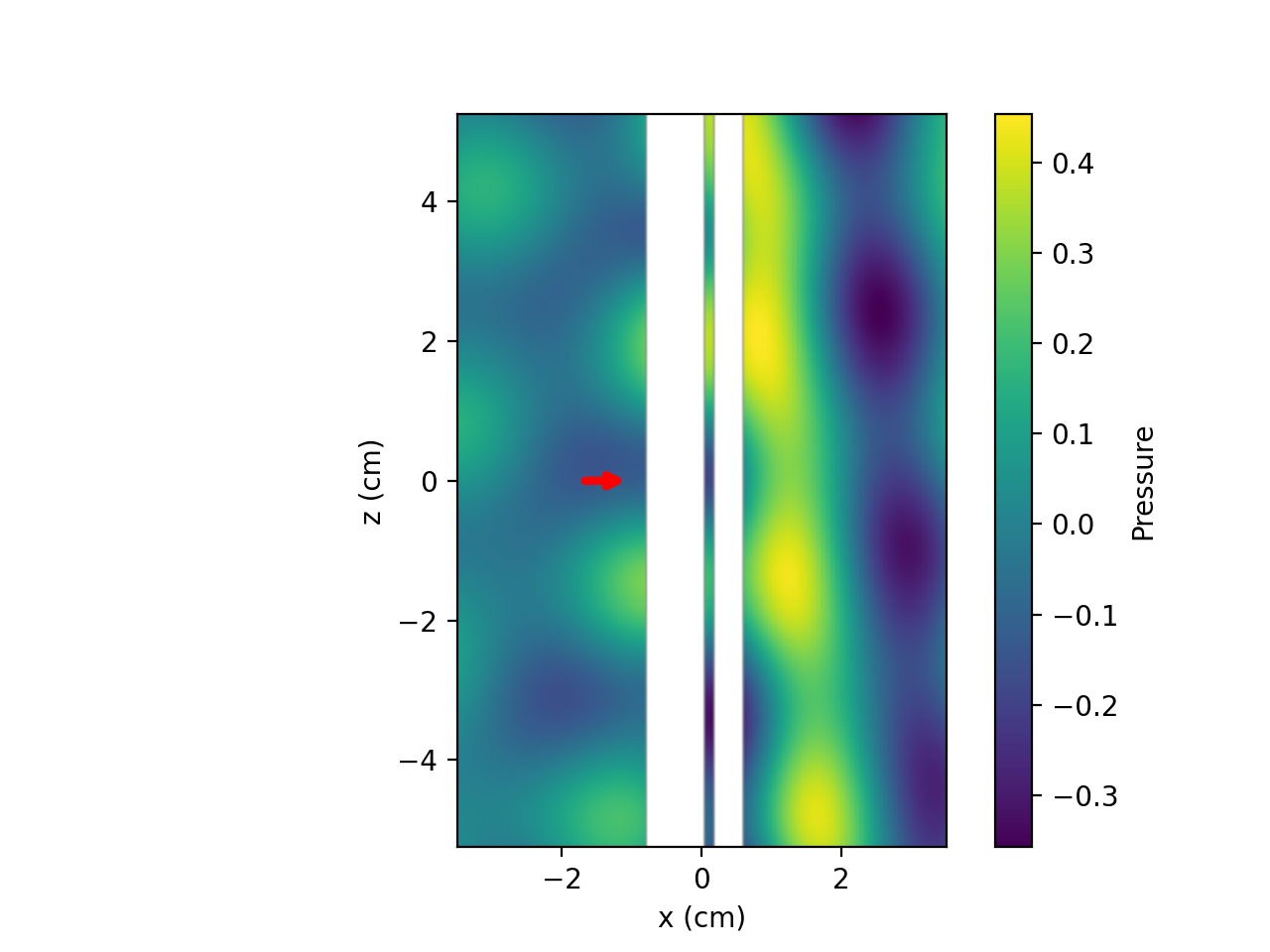
and plot the results.

(Source code)

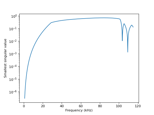
Two-dimensional arrays (in the xy plane)

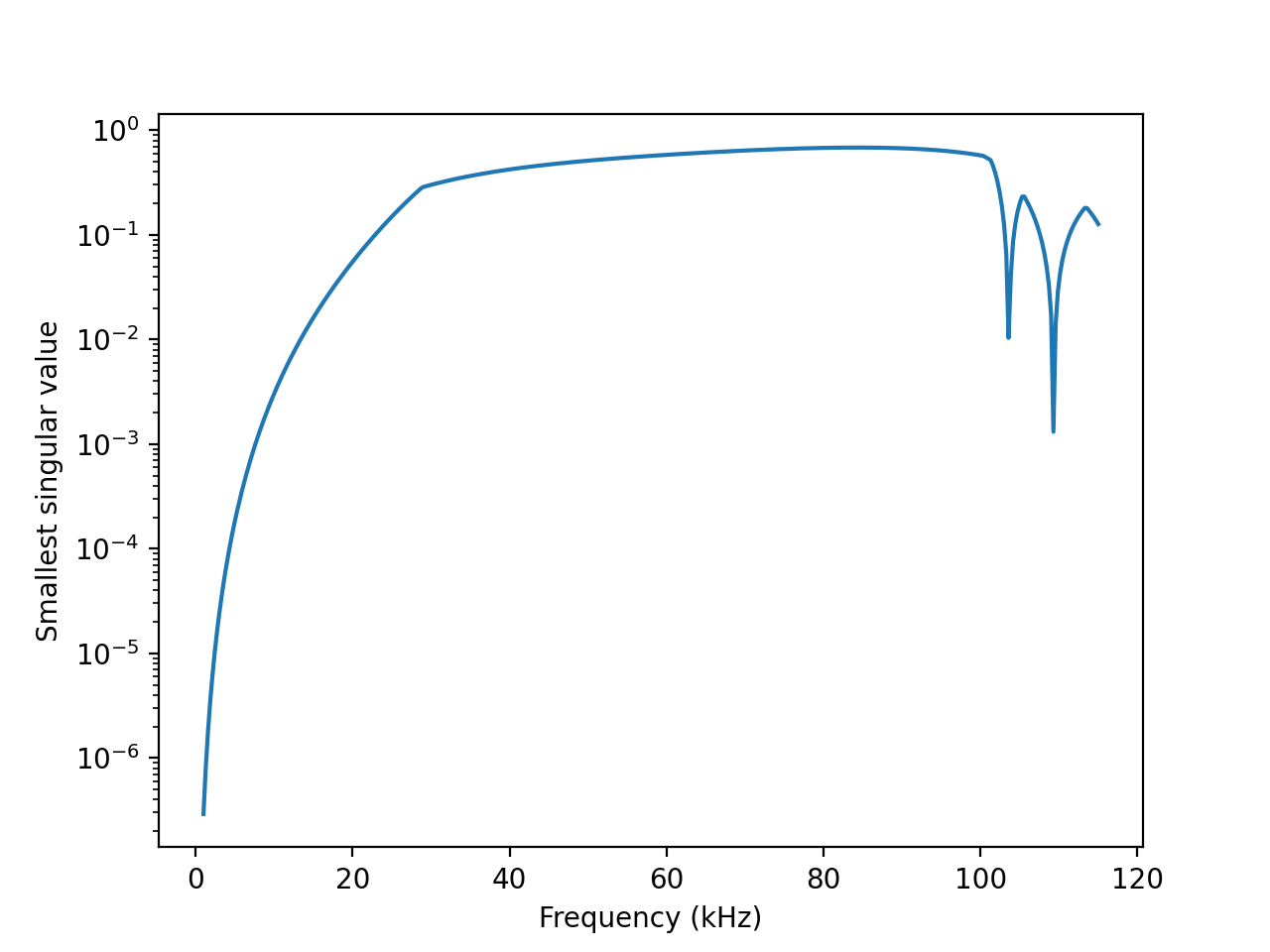
As the last example, let us examine a structure that is a crystal consisting of infinitely long cylinders in a square array in the xy plane.

k0s = 2 * np.pi * np.linspace(1000, 115000, 400) / 343
materials = [acoustotreams.AcousticMaterial(1050, 2350), acoustotreams.AcousticMaterial(998, 1497)]
mmax = 6
radius = 0.005
lattice = acoustotreams.Lattice.cubic(0.015)
kpar = [0, 0, 0]

def compute_svd(k0):
    cyl = acoustotreams.AcousticTMatrixC.cylinder(kpar[2], mmax, k0, radius, materials)
    svd = np.linalg.svd(cyl.latticeinteraction(lattice, kpar[:2]), compute_uv=False)
    return svd[-1]
res = Parallel(n_jobs=-1)(delayed(compute_svd)(k0s[i]) for i in range(len(k0s)))

fig, ax = plt.subplots()
ax.set_xlabel("Frequency (kHz)")
ax.set_ylabel("Smallest singular value")
ax.semilogy(343 * k0s / (2 * np.pi) / 1000, res)
fig.show()

Similarly to the case of spheres and a three-dimensional lattice, we can check the smallest singular value.

(Source code, png, hires.png, pdf)