Acoustic T-Matrices
One of the main objects for acoustic scattering calculations within acoustotreams are acoustic T-matrices. They describe the scattering response of an object by encoding the linear relationship between incident and scattered fields. These fields are expanded using the scalar spherical waves.
The acoustic T-matrices of spheres can be obtained analytically. For more complicated shapes numerical methods are necessary to compute the acoustic T-matrix. Once the T-matrix of a single object is known, the acoustic interaction between particle within clusters can be calculated efficiently. Such clusters can be analyzed in their local description, where the field expansions are centered at each particle of the cluster, or in a global description treating the whole cluster as a single object.
acoustotreams is particularly aimed at analyzing scattering within lattices. These lattices can be periodic in one, two, or all three spatial dimensions. The unit cell of those lattices can consist of an arbitrary number of objects described by the acoustic T-matrix.
Spheres
It’s possible to calculate the acoustic T-matrix of a single sphere with the
method sphere(). We start by defining the relevant parameters for
our calculation and creating the acoustic T-matrices themselves.
k0s = 2 * np.pi * np.linspace(50000, 500000, 200) / acoustotreams.AcousticMaterial().c
materials = [acoustotreams.AcousticMaterial(1050 + 100j, 2350 - 300j),
             acoustotreams.AcousticMaterial(998, 1497)]
lmax = 10
radius = 0.005
spheres = [acoustotreams.AcousticTMatrix.sphere(lmax, k0, radius, materials) for k0 in k0s]
Here we define a material using the class AcousticMaterial().
To create an instance of this class, we pass three arguments: mass density,
longitudinal speed of sound, and transverse speed of sound. The acoustic
material parameters can be complex. The imaginary part of the density must be
positive, whereas the imaginary part of the speeds negative.
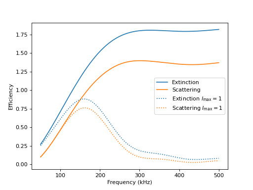
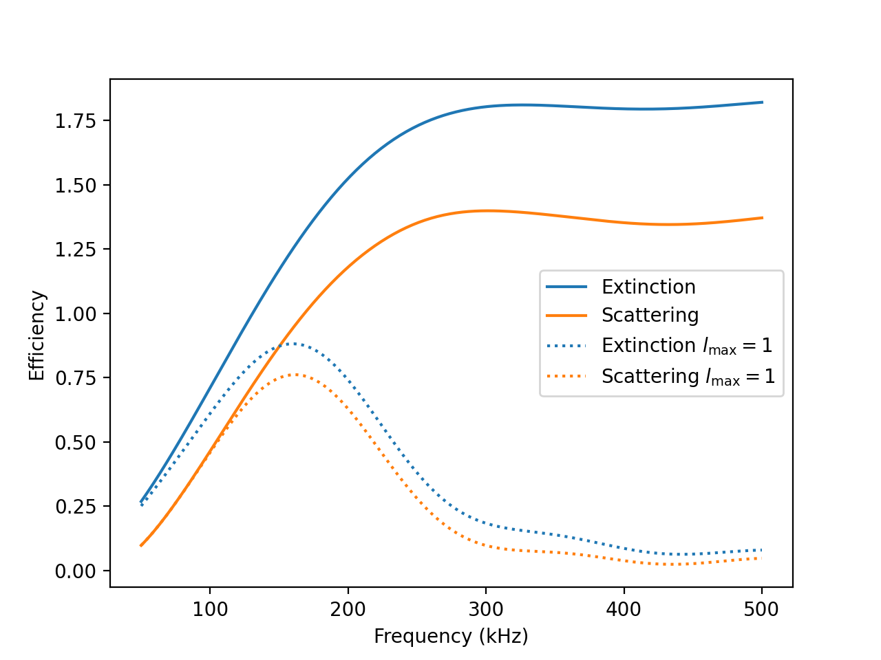
Now, we can easily access quantities like the scattering and extinction cross sections
xs_sca = np.array([tm.xs_sca_avg for tm in spheres]) / (np.pi * radius ** 2)
xs_ext = np.array([tm.xs_ext_avg for tm in spheres]) / (np.pi * radius ** 2)
From the parameter lmax = 10 we see that the acoustic T-matrix is calculated up to the tenth
multipolar order. To restrict the T-matrix in the monopole-dipole approximation, we can
select a basis containing only those multipoles.
swb_lmax1 = acoustotreams.ScalarSphericalWaveBasis.default(1)
spheres_lmax1 = [tm[swb_lmax1] for tm in spheres]
xs_sca_lmax1 = np.array([tm.xs_sca_avg for tm in spheres_lmax1]) / (np.pi * radius ** 2)
xs_ext_lmax1 = np.array([tm.xs_ext_avg for tm in spheres_lmax1]) / (np.pi * radius ** 2)
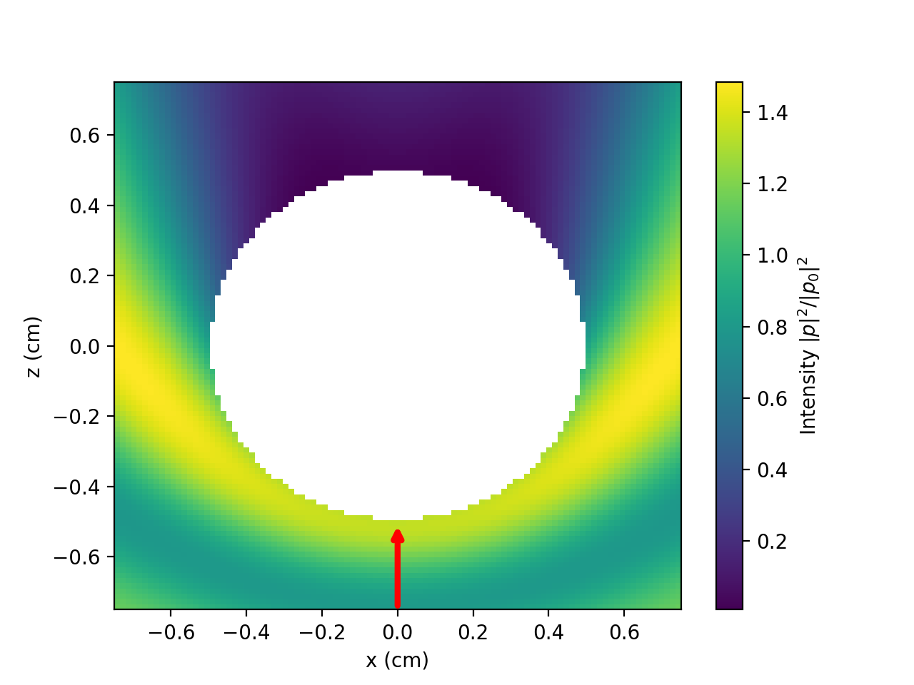
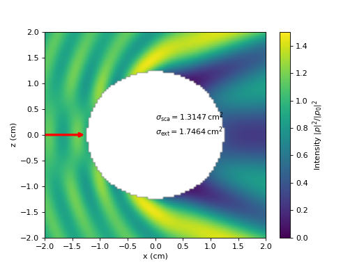
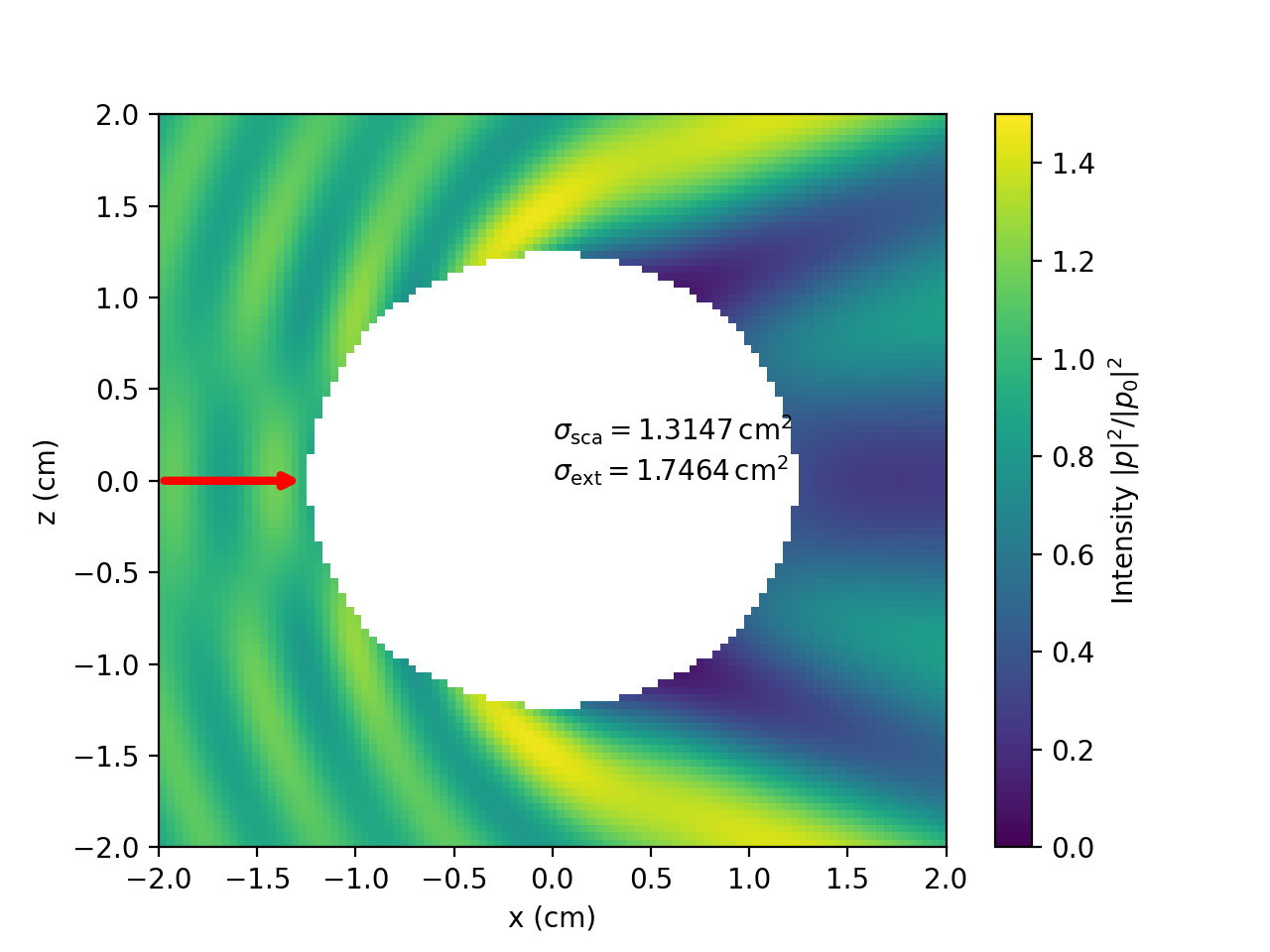
Now, we can look at the results by plotting them and observe, unsurprisingly, that for larger frequencies the monopole-dipole approximation is not giving an accurate result. Further, we visualize the total acoustic field intensity at frequency 163 kHz.
tm = spheres[50]
inc = acoustotreams.plane_wave_scalar([0, 0, tm.k0], k0=tm.k0, material=tm.material)
sca = tm.sca(inc)
x = np.linspace(-0.0075, 0.0075, 101)
z = np.linspace(-0.0075, 0.0075, 101)
def compute_intensity(i, j):
    r = [x[j], 0, z[i]]
    result = 0
    if tm.valid_points(r, [radius]):
        result = np.abs(inc.pfield(r) + sca.pfield(r))**2
    else:
        result = np.nan
    return i, j, result
results = Parallel(n_jobs=-1)(
    delayed(compute_intensity)(i, j) for i in range(len(z)) for j in range(len(x))
)
intensity = np.zeros((len(z), len(x)))
for i, j, result in results:
    intensity[i, j] = result
We select the T-matrix and illuminate it with a plane wave. Next, we set up
the x and z coordinates and define the auxiliary function to compute
the intensity at a single valid point. We can calculate the intensity
of the fields as a superposition of incident and scattered fields.
Here, we also accelerate the computations using paralyzation by
Parallel in joblib.
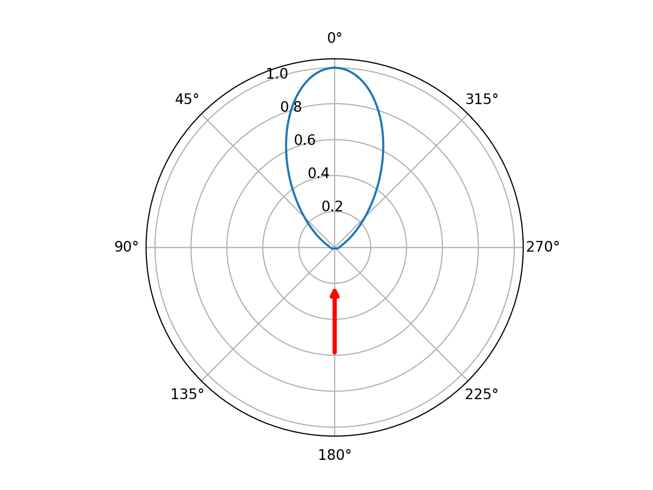
Finally, we compute the radiation pattern of the sphere at the same frequency as a function of the polar angle \(\theta\). The red arrow indicates the direction of incidence of the plane wave.
theta = np.linspace(0, 2 * np.pi, 301)
radpattern = np.zeros(len(theta))
def compute_radpattern(i):
    n = [np.sin(theta[i]), 0, np.cos(theta[i])]
    return np.abs(sca.pamplitudeff(n))**2
radpattern = Parallel(n_jobs=-1)(delayed(compute_radpattern)(i) for i in range(len(theta)))


Clusters
Multi-scattering calculations in a cluster of particles is a typical application of the T-matrix method. We first construct an object from two spheres. Using the definition of the relevant parameters
k0 = 2 * np.pi * 150000 / acoustotreams.AcousticMaterial().c
materials = [acoustotreams.AcousticMaterial(1050 + 100j, 2350 - 300j),
             acoustotreams.AcousticMaterial(998, 1497)]
lmax = 3
radii = [0.005, 0.005]
positions = np.array(
    [
        [0.0075, 0, 0],
        [-0.0075, 0, 0],
    ]
)
we can simply first create the spheres and put them together in a cluster, where we immediately calculate the interaction.
spheres = [acoustotreams.AcousticTMatrix.sphere(lmax, k0, r, materials) for r in radii]
tm = acoustotreams.AcousticTMatrix.cluster(spheres, positions).interaction.solve()
Then, we can illuminate with a plane wave and get the scattered field coefficients and the scattering and extinction cross sections for that particular illumination.
inc = acoustotreams.plane_wave_scalar([0, 0, tm.k0], k0=tm.k0, material=tm.material)
sca = tm.sca(inc)
xs = tm.xs(inc)
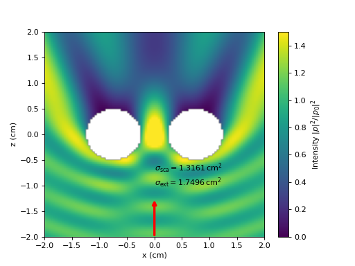
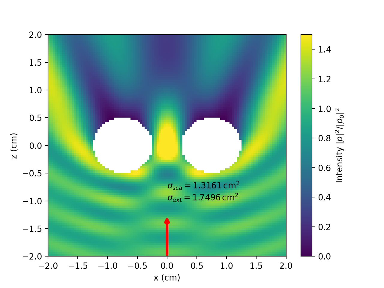
Finally, with few lines similar to the plotting of the field intensity of a single sphere we can obtain the fields outside of the sphere.
x = np.linspace(-0.02, 0.02, 101)
z = np.linspace(-0.02, 0.02, 101)
def compute_intensity(i, j, tm, radii, inc, sca):
    r = [x[j], 0, z[i]]
    result = 0
    if tm.valid_points(r, radii):
        result = np.abs(inc.pfield(r) + sca.pfield(r))**2
    else:
        result = np.nan
    return i, j, result
results = Parallel(n_jobs=-1)(
    delayed(compute_intensity)(i, j, tm, radii, inc, sca)
    for i in range(len(z))
    for j in range(len(x))
)
intensity = np.zeros((len(z), len(x)))
for i, j, result in results:
    intensity[i, j] = result
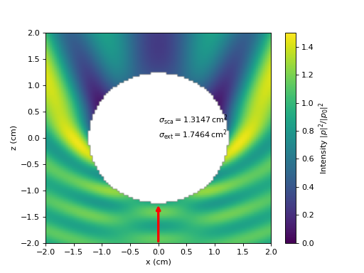
Up to here, we did all calculations for the cluster in the local basis. By expanding the incident and scattered fields in a basis with a single origin we can describe the same object. Often, a larger number of multipoles is needed to do so and some information on fields between the particles is lost. However, the description in a global basis can be more efficient in terms of matrix size.
tm_global = tm.expand(acoustotreams.ScalarSphericalWaveBasis.default(10))
sca = tm_global.sca(inc)
A comparison of the calculated near-fields and the cross sections show good agreement between the results of both, local and global, T-matrices.
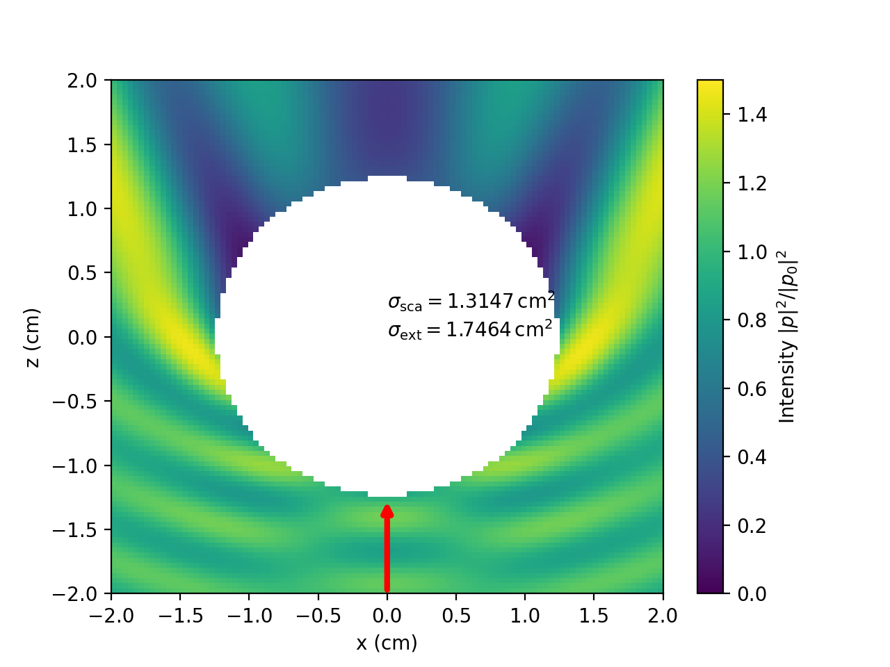
In the last figure, the T-matrix is rotated by 90 degrees about the y axis and the illumination is set accordingly to be a plane wave propagating in the x direction, such that the whole system remains the same. It shows how the rotate operator produces consistent results.
inc = acoustotreams.plane_wave_scalar([k0, 0, 0], k0=tm.k0, material=tm.material)
tm_rotate = tm_global.rotate(0, np.pi / 2)

One-dimensional arrays (along z)
Next, we turn to systems that are periodic in the z direction. We calculate the scattering from an array of spheres. Intentionally, we choose a unit cell with two different spheres that overlap along the z direction, but are not placed exactly along the same line. This is the most general case for the implemented lattice sums. After the common setup of the parameters, we simply create a cluster in a local basis.
k0 =  2 * np.pi * 50000 / acoustotreams.AcousticMaterial().c
materials = [acoustotreams.AcousticMaterial(1050 + 100j, 2350 - 300j),
            acoustotreams.AcousticMaterial(998, 1497)]
lmax = 3
radii = [0.0075, 0.0065]
positions = [[-0.004, 0, -0.0075], [0.004, 0, 0.0075]]
period = 0.035
lattice = acoustotreams.Lattice(period)
kz = 0
This time we let them interact specifying a one-dimensional lattice, so that the spheres form a chain.
spheres = [acoustotreams.AcousticTMatrix.sphere(lmax, k0, r, materials) for r in radii]
chain = acoustotreams.AcousticTMatrix.cluster(spheres, positions).latticeinteraction.solve(lattice, kz)
Next, we choose set the illumination to be propagating along the x axis. The z component of the wave vector of the plane wave has to match to the wave vector component of the lattice interaction, i.e., the Bloch wave vector.
inc = acoustotreams.plane_wave_scalar([chain.k0, 0, 0], k0=chain.k0, material=chain.material)
sca = chain.sca(inc)
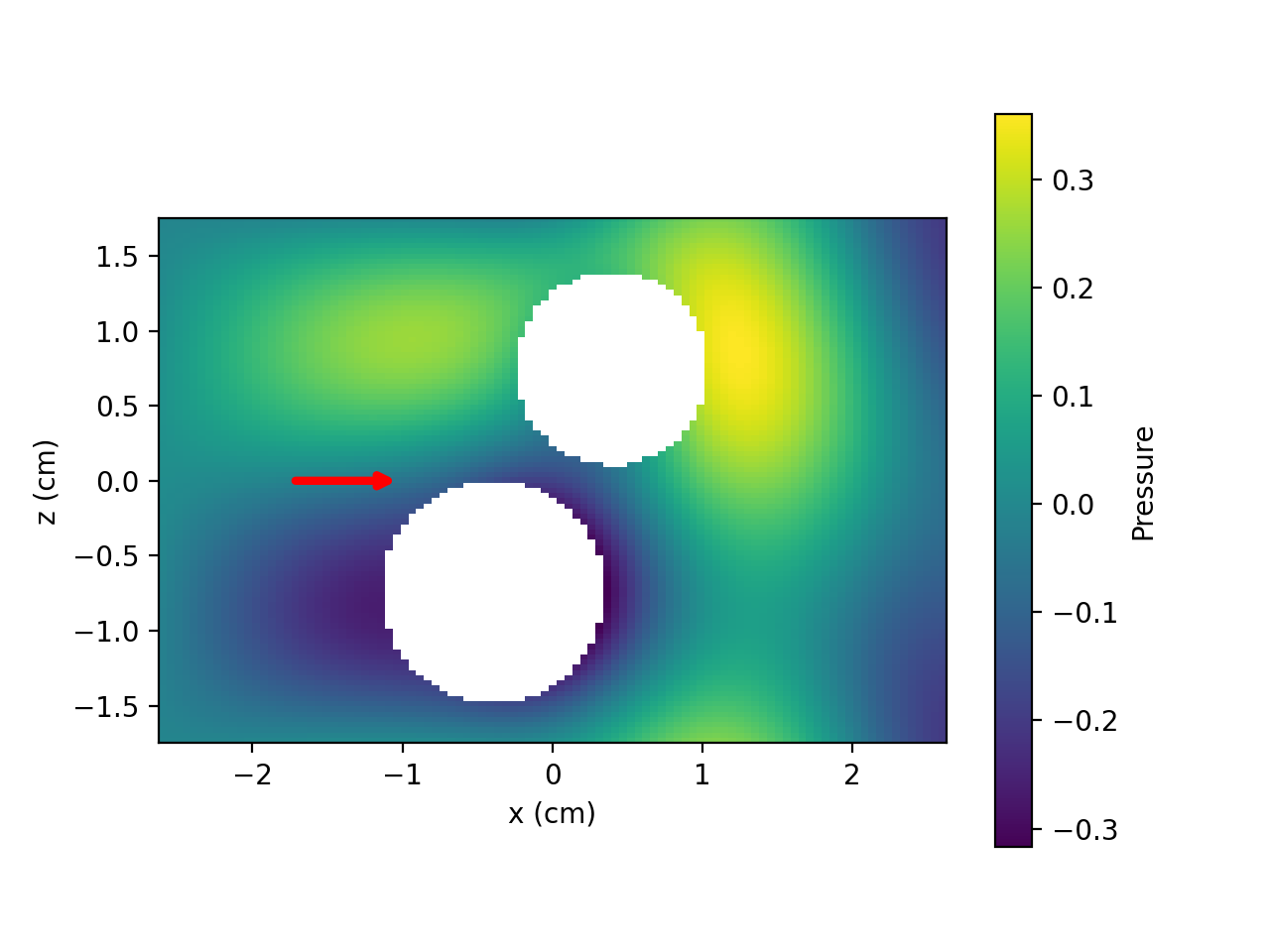
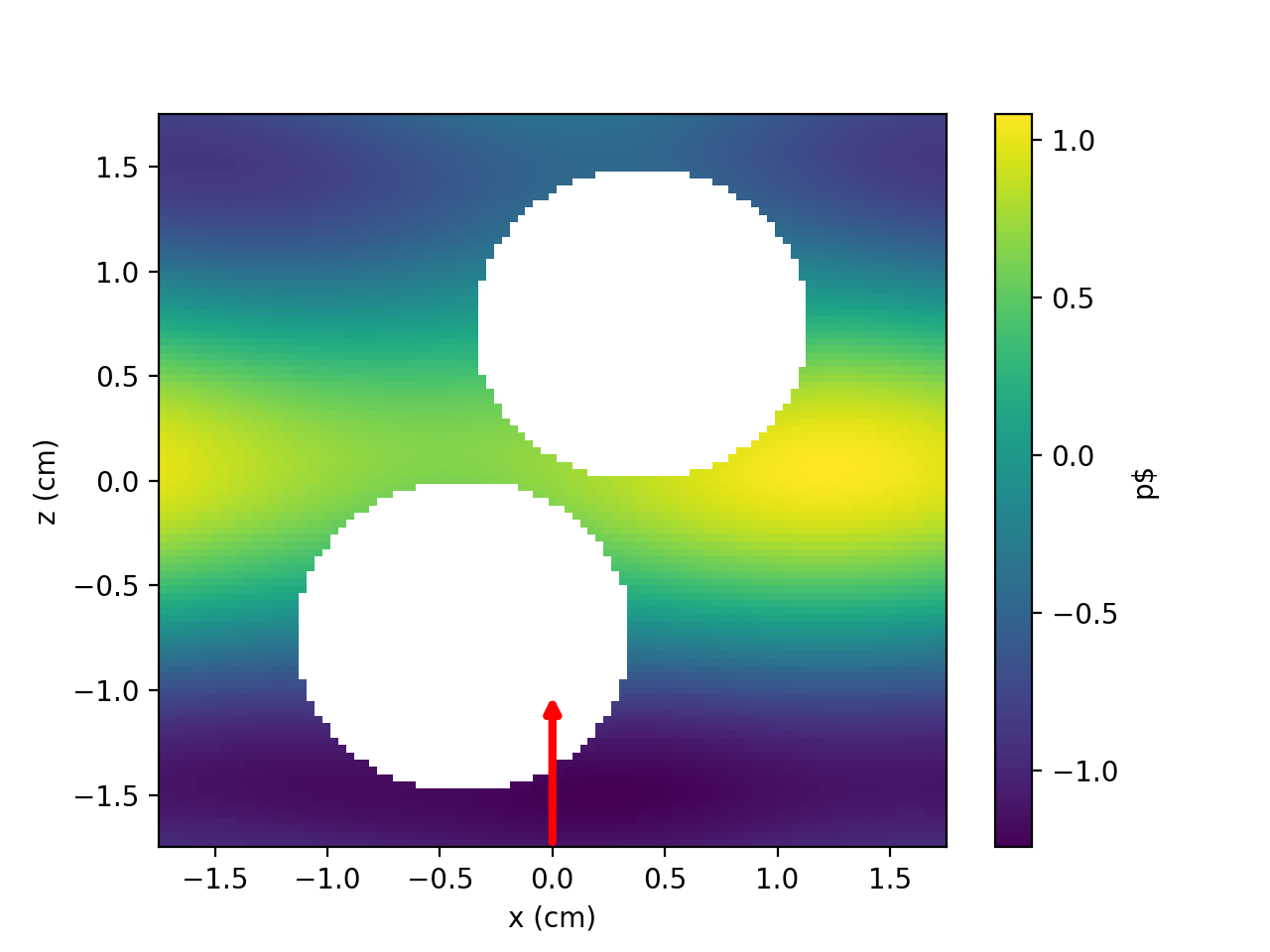
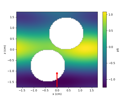
There is an efficient way to calculate the acoustic response, especially in the far-field, using cylindrical acoustic T-matrices. That will be introduced in Acoustic cylindrical T-Matrices. Here, we will stay in the expression of the fields as scalar spherical waves. This allows the calculation of the fields in the domain between the spheres. To compute them accurately, we expand the scattered field coefficients in the whole lattice in monopole approximation at each point we want to calculate the pressure field.
x = np.linspace(-0.75 * period, 0.75 * period, 101)
z = np.linspace(-0.5 * period, 0.5 * period, 101)
def compute_pressure(i, j):
    r = [x[j], 0, z[i]]
    if chain.valid_points(r, radii):
        swb = acoustotreams.ScalarSphericalWaveBasis.default(0, positions=[r])
        result = sca.expandlattice(basis=swb).pfield(r)
    else:
        result = np.nan
    return i, j, result
results = Parallel(n_jobs=-1)(
    delayed(compute_pressure)(i, j)
    for i in range(len(z))
    for j in range(len(x))
)
p = np.zeros((len(z), len(x)), complex)
for i, j, result in results:
    p[i, j] = result
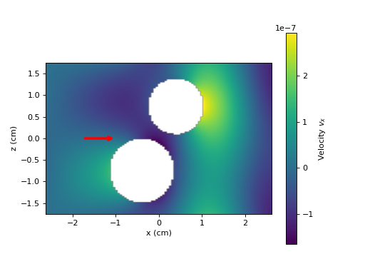
To calculate the velocity field, we again expand the scattered field coefficients, however, in the dipole approximation.
def compute_velocity(i, j):
    r = [x[j], 0, z[i]]
    if chain.valid_points(r, radii):
        swb = acoustotreams.ScalarSphericalWaveBasis.default(1, positions=[r])
        result = sca.expandlattice(basis=swb).vfield(r)[0]
    else:
        result = np.nan
    return i, j, result
results = Parallel(n_jobs=-1)(
    delayed(compute_velocity)(i, j)
    for i in range(len(z))
    for j in range(len(x))
)
vx = np.zeros((len(z), len(x)), complex)
for i, j, result in results:
    vx[i, j] = result
(Source code, png, hires.png, pdf)

Two-dimensional arrays (in the xy plane)
The case of periodicity in two directions is similar to the case of the previous section with one-dimensional periodicity. Here, by convention the array has to be in the xy plane.
k0 =  2 * np.pi * 50000 / acoustotreams.AcousticMaterial().c
materials = [acoustotreams.AcousticMaterial(1050 + 100j, 2350 - 300j),
            acoustotreams.AcousticMaterial(998, 1497)]
lmax = 3
radii = [0.0075, 0.0075]
positions = [[-0.004, 0, -0.0075], [0.004, 0, 0.0075]]
period = 0.035
lattice = acoustotreams.Lattice.square(period)
kpar = [0, 0]

spheres = [acoustotreams.AcousticTMatrix.sphere(lmax, k0, r, materials) for r in radii]
array = acoustotreams.AcousticTMatrix.cluster(spheres, positions).latticeinteraction.solve(
    lattice, kpar
    )
inc = acoustotreams.plane_wave_scalar([0, 0, array.k0], k0=array.k0, material=array.material)
sca = array.sca(inc)

x = np.linspace(-0.5 * period, 0.5 * period, 101)
z = np.linspace(-0.5 * period, 0.5 * period, 101)
def compute_intensity(i, j, tm, radii, inc, sca):
    r = [x[j], 0, z[i]]
    if tm.valid_points(r, radii):
        swb = acoustotreams.ScalarSphericalWaveBasis.default(0, positions=[r])
        field = sca.expandlattice(basis=swb).pfield(r)
        result = np.real(inc.pfield(r) + field)
    else:
        result = np.nan
    return i, j, result
results = Parallel(n_jobs=-1)(
    delayed(compute_intensity)(i, j, array, radii, inc, sca)
    for i in range(len(z))
    for j in range(len(x))
)
intensity = np.zeros((len(z), len(x)))
for i, j, result in results:
    intensity[i, j] = result
With a few changes we computed the fields in a square array of the same spheres as in the
previous examples. Most importantly we changed the value of the variable lattice
to an instance of a two-dimensional Lattice and set kpar
accordingly. Most other changes are just resulting from the change of the coordinate
system.
(Source code, png, hires.png, pdf)
Three-dimensional arrays
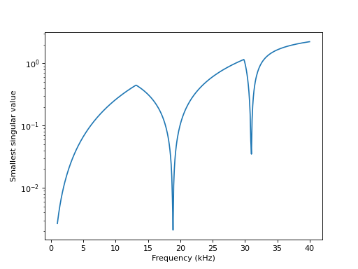
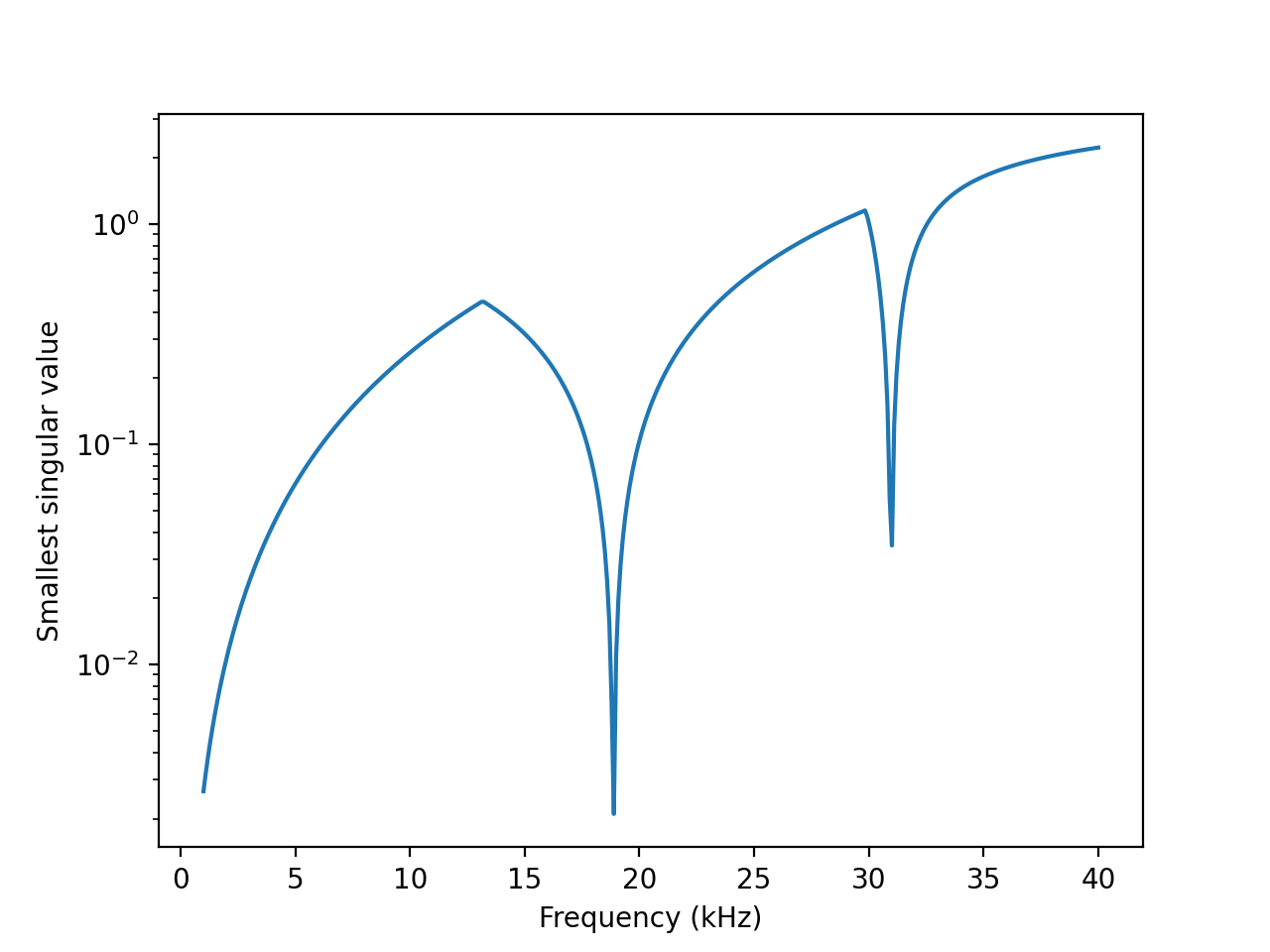
In a three-dimensional lattice we are mostly concerned with finding eigenmodes of a crystal. We want to restrict the example to calculating modes at the gamma point in reciprocal space. The calculated system consists of a single sphere in a cubic lattice. In our very crude analysis, we blindly select the lowest singular value of the lattice interaction matrix. Besides the mode when the frequency tends to zero, there are two additional modes at higher frequencies in the chosen range.
k0s = 2 * np.pi * np.linspace(1000, 40000, 400) / acoustotreams.AcousticMaterial().c
materials = [acoustotreams.AcousticMaterial(1050, 2350), acoustotreams.AcousticMaterial(998, 1497)]
lmax = 3
radius = 0.005
lattice = acoustotreams.Lattice.cubic(0.015)
kpar = [0, 0, 0]

def compute_svd(k0):
    sphere = acoustotreams.AcousticTMatrix.sphere(lmax, k0, radius, materials)
    svd = np.linalg.svd(sphere.latticeinteraction(lattice, kpar), compute_uv=False)
    return svd[-1]
res = Parallel(n_jobs=-1)(delayed(compute_svd)(k0s[i]) for i in range(len(k0s)))
(Source code, png, hires.png, pdf)
